Explaining the important bias variance tradeoff problem in classical machine learning and its contradiction with modern deep learning
Some philosophy
As you probably know, machine learning is a type of process where we take a computing machine (a computer) and teach it to do some complex things. But what the hell does “teach” really mean and actually, what is considered “complex” enough?
Well, the tough truth is that we don’t know. A complex problem is mainly considered a problem that is tough to learn via a standard programming procedure – lets keep it at that. But still, what do we mean by teaching the computer? After all we just gave it a sequence of commands to do and it followed them perfectly – without doing anything by itself. After the learning process the computer still only does the same things: it has the same architecture, the same set of commands and the same hardware specifications as before.
This discussion can be the starting ground to deeper philosophical arguments about the nature of learning and the acquirement of skills in general. For the sake of our sanity – we are going to gloss over this discussion (even though it is interesting).

“Teaching” a machine
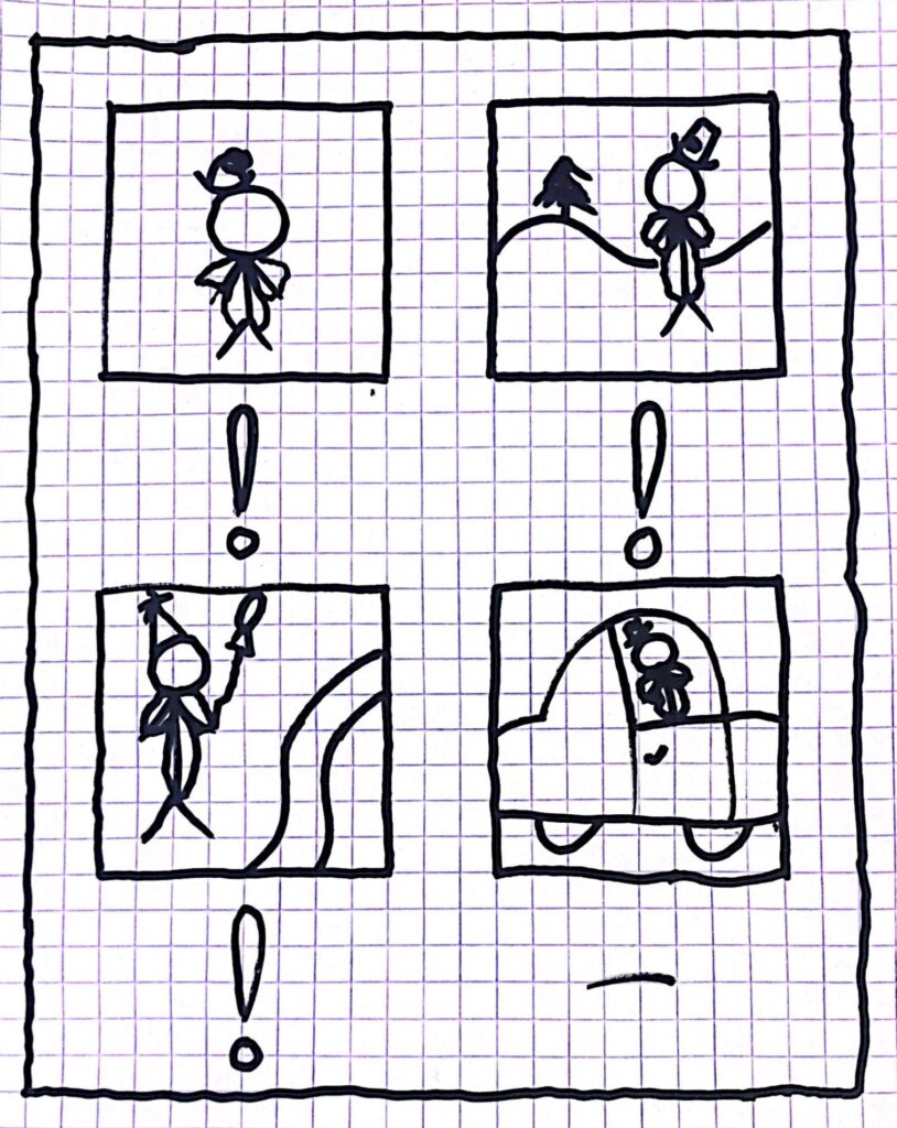
For now we are going to focus on machine learning and more specifically – when we say “teach” a machine to a task of some sort, what exactly did we teach it? For example, let’s say our task is that our computer needs to print a “!” sign every time we give it a picture of a clown and do nothing otherwise. It might be the case that after the learning period, the computer successfully identifies the clown in the first three photos, but in the fourth picture it didn’t. What was special about the fourth picture? The clown was driving a car.
An obvious questions is: What exactly did our computer learn here? Did our computer learn how to identify a clown or did it learn how to identify a “standing outside clown”?
In order to understand what is happening here and why, we need to understand how computers “learn”.
There is a saying: “If you give a computer a fish, it will know it’s a fish, if you give it another one, it won’t”. Although it’s amusing, this can be quite true. You see, the way computers (generally) learn is by giving them lots of examples. In our case, we showed the computer a lot of images, ones with and without clowns. After each picture the computer analyzed, we told it if it was right or wrong. Over time, by learning from a lot of examples the computer learned what to do.
A simpler problem
Computer vision is a pretty complicated task, so in order to understand the driving clown problem we will take an interlude into a simpler task. Let’s say we have a set of points belonging to a polynomial p(x) and we want the computer to identify p. So, after the computer learns we expect that if we give it some value x it will give us p(x).
This seems pretty straightforward. After all if p is of degree n then the Fundamental Theorem of algebra tells us that given at least n of these points we can determine p exactly – and the computer can too. The problem is that our world is not perfect and there is noise everywhere. In a computer vision task the noise can come from many sources: the lighting in the room, the positioning of certain lamps or the sun, the angle of certain objects and even the shape of the camera lens or the file format of the picture. Some of the noise is significant and some is pretty negligible, but one thing is certain – there will always be noise.

If we include noise in our problem then the points change their values as in:
\{(x_i,p(x_i))|i\in[10]\}\rightarrow\{(x_i,p(x_i)+\varepsilon_i)|i\in[10],\varepsilon_i\sim\mathcal{N}(\mu,\sigma^2)\}
where \mathcal{N} is a normal distribution with some average, \mu, close to zero and a small standard deviation \sigma. The larger the parameters of the distribution the noise is sampled from – the harder it will be to learn the underlying polynomial.
In the end, our algorithm needs to guess a polynomial of the type p(x)=\sum_{k=0}^{N}{a_kx^k}, we just need to help it learn the right values of the coefficients. At the start, the model doesn’t really know anything about the polynomial, except that its values are close to the ones at the given points. Particularly it doesn’t know the value of N – the degree of the polynomial. In other words, the computer doesn’t know how complex the polynomial is, if it is a straight line, a parabola or 17x^{161}-16x^{27}+3, it has no way to tell. What value of N should our model pick? How many parameters should it learn?
The bias variance tradeoff
The bright reader might notice that if the real polynomial’s degree is N_r but the computer’s is N_c and N_c<N_r then at large values of x the learned polynomial will be far off from the real one. On the other hand if N_c\geq N_r then we still have the ability to learn the exact same polynomial – give the last coefficients a value of zero. So, should we have N_c=\infty? This is impossible since we will have to learn infinitely many parameters. OK, so not infinity, but should we make N_c as big as we can so that we could always in theory learn the real polynomial? Well, the simple answer is… NO! And here is why.
Bias, Variance and the tradeoff between them
A data scientist that would make N_c as big as possible takes exclusive care of the bias of the problem. You can think of the bias as the magnitude of the error of the computer’s optimal solution compared to the real solution. For example, if the model uses N_c=1 and it needs to learn a parabola then the model’s bias will be the difference between the parabola and the straight line closest to it.
In the polynomial problem case, the bias is higher if N_c is smaller – since if the degree of the polynomial is smaller, the computer can learn only simpler solutions, and it will be farther off from complex polynomials that can be the real solutions. But this is not good enough – we want the optimal solution to be the real solution! We want the bias to be zero. But a bias of zero comes at a cost – and that cost’s name is variance.
You can think of the variance as the computer’s sensitivity to noise. In the polynomial problem above, the variance is the sensitivity of the computer’s learning process to the values of \varepsilon_i – the noise in the points’ values. We can notice that if N_c is larger than the variance will be greater. If N_c is larger then the computer will guess more complex polynomials. This means that the computer will have more options to choose from, specifically, it will have more options that are closer to the points’ values. Because the values are affected by the noise, and because the computer will get closer and closer to them, the computer will be affected more by the noise if N_c is larger. When a model has high variance we say that it is “overfitting” to the training data, it doesn’t generalize it enough to get rid of the noise.
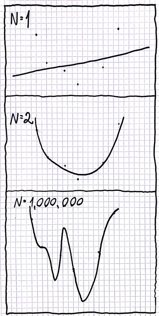
Which case is closest to the parabola? Which is closest to the sample points?
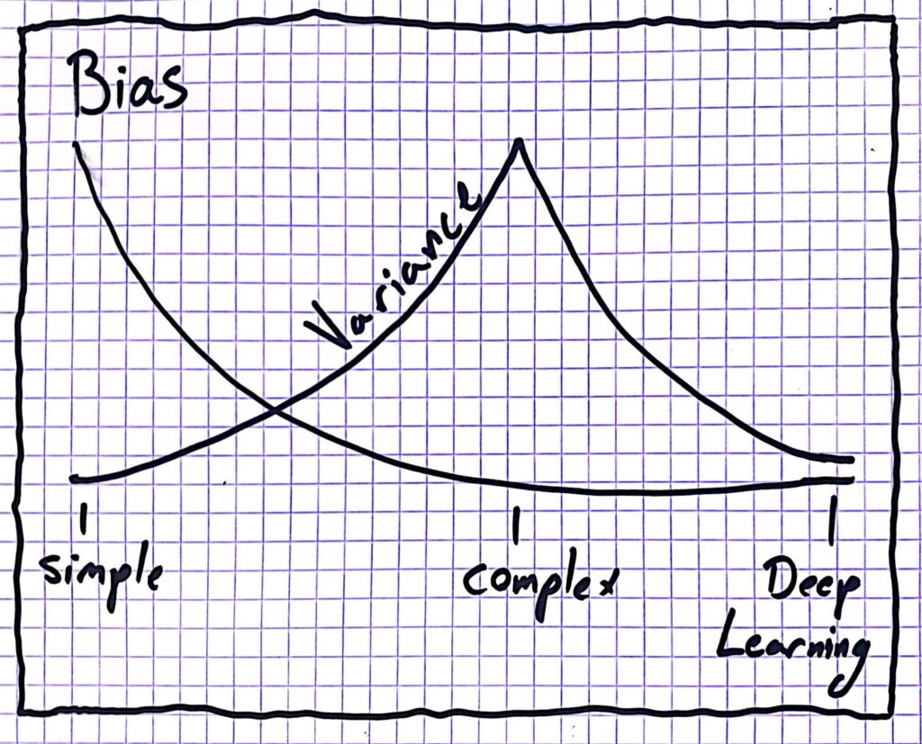
So, to conclude, if we have a larger value for N_c\ \rightarrow we have a more complex model \rightarrow smaller bias. But in addition to that a large N_c\ \rightarrow more sensitivity to noise \rightarrow larger variance. This is the famous bias variance tradeoff.
Implications of the tradeoff
This doesn’t give us a simple solution to our problem. If we train a complex model then the variance will be higher, if we train a simpler model then the bias will be higher. In both cases we either have the bias or the variance pushing us away from predicting the correct solution. We should pick something in between, a model that is complex enough but not too complex (a middle value for N_c). Our goal is to minimize both the bias and the variance – that essentially is the entire goal of machine learning.
Back to the image processing problem of the clowns. Our model could most of the time predict one standing, but not sitting in a car. The clown sitting in a car was a legitimate example, it was a legitimate “point of the polynomial” and the car wasn’t there because of any sort of noise. The fact that our model couldn’t predict the outcome of this legitimate input tells us that it wasn’t complex enough – the bias was too high. On the other hand, if we gave the model a slightly darker version of a clown standing and he wouldn’t be able to recognize it, this means that the variance was too high – the model was too sensitive to the lighting (which is a noise factor).
Notice that if we gave our model more examples to learn from, for example if we give him a picture of a clown sitting in a car or dark versions of a clown standing it would probably be better at predicting both, just like if we give more points to our polynomial predictor. This means that there is a way to get both bias and variance down together – gather and learn on more data. This “trick” works both on simple and on complex learning models.
A contradiction with deep learning
Another amazing kind of unexplained phenomenon in machine learning is the success of deep learning. In deep learning we make the model extremely complex. Think of it as taking N_c to be an absurdly large value, hence the variance is supposed to be very high. But the weird thing is, it is not. If we design models that heuristically make sense such as deep Convolutional or Recurrent neural networks (the fancy terms don’t really matter right now) then we get to a magic region where the bias goes down because the model is more expressive but the variance doesn’t go up. As a consequence large companies construct gigantic models that perform better, but our understanding of why this works is still lagging behind. According to the time this article was written, this phenomenon is unexplained and remains a mystery.
If someone finds a proof that explains why and how this happens, maybe we will know the limitations and capabilities of our current methods in machine learning. Furthermore, if the proof will be constructive, maybe we will be able to find a “sweet spot” that will help us determine the best complexity for a given learning task (i.e. the best value of N_c). It might be the case that after a real understanding of this topic people will stop being afraid of AI taking over the world. But on the other hand, maybe the findings will just reinforce their unease.